Assignment 1
In this assignment, we will dive into transformations. It’s important that you get how to apply transformations to objects in 3D scenes and how to compose transformations, as you will use these operations a lot in the final assignment of this course. In this assignment, we slowly build up complexity: first, you will create transformation matrices from scratch to control a virtual car. Then you will compose transformation matrices to construct a lamp. Finally, you can apply these lessons to build an animated solar system. Follow the comments in ex01.py and ex02.py to finish the assignments. You can use this document as a reference. There are questions in this document. Don’t skip over them, but think about them. If you can’t answer them, feel free to ask one of the TAs.
Translation matrices
You have learned about translation matrices and how they can be applied in order to move points in space. Below you can see how a point is moved by multiplying with a translation matrix
\[\begin{bmatrix} 1 & 0 & 0 & t_x \\ 0 & 1 & 0 & t_y \\ 0 & 0 & 1 & t_z \\ 0 & 0 & 0 & 1 \\ \end{bmatrix} \begin{bmatrix} v_x \\ v_y \\ v_z \\ 1 \end{bmatrix} = \begin{bmatrix} v_x + t_x \\ v_y + t_y \\ v_z + t_z\\ 1 \end{bmatrix}.\]$\rightarrow$ Why are we using four dimensions in the matrix and
coordinates of the point?
$\rightarrow$ Can you compute the result yourself?
$\rightarrow$ What would happen to the result if the last entry in the
matrix was a 4?
In the translate function you see that we create a matrix mat which will become your translation matrix. You must fill in the rows and columns of this matrix appropriately to form such a matrix. It starts off as the identity matrix
\[\begin{bmatrix} 1 & 0 & 0 & 0 \\ 0 & 1 & 0 & 0 \\ 0 & 0 & 1 & 0 \\ 0 & 0 & 0 & 1 \\ \end{bmatrix}\]Rotation matrices
We use a rotation matrix to rotate points. In 3D, a point can be rotated around three possible axes (the x, y and z axes). Therefore, we need three rotation matrices to support all these rotations.
\[R_x(\theta) = \begin{bmatrix} 1 & 0 & 0 \\ 0 & \cos{\theta} & -\sin{\theta} \\ 0 & \sin{\theta} & \cos{\theta} \\ \end{bmatrix}\] \[R_y(\theta) = \begin{bmatrix} \cos{\theta} & 0 & \sin{\theta} \\ 0 & 1 & 0 \\ -\sin{\theta} & 0 & \cos{\theta} \\ \end{bmatrix}\] \[R_z(\theta) = \begin{bmatrix} \cos{\theta} & -\sin{\theta} & 0 \\ \sin{\theta} & \cos{\theta} & 0 \\ 0 & 0 & 1 \\ \end{bmatrix}\]Composing transformations
Let’s say you want to rotate a point and then translate it. You have created the rotation matrix $\mathbf{R}$ and translation matrix $\mathbf{T}$. The point you want to transform is called $\mathbf{p}$. You could first compute the rotation \[\mathbf{p}’ = \mathbf{Rp}\] and then the translation \[\mathbf{p}’’ = \mathbf{Tp}’.\] Another way to write this is \[\mathbf{p}’ = \mathbf{TRp}.\] You could also first compute the product of the matrices $\mathbf{T}$ and $\mathbf{R}$ and then multiply the result with $\mathbf{p}$.
\[\begin{aligned} \mathbf{M} = \mathbf{TR} \\ \mathbf{p}' = \mathbf{Mp}. \end{aligned}\]This is possible, because matrix products are associative, a fancy word to say that $(\mathbf{AB})\mathbf{C} = \mathbf{A}(\mathbf{BC})$. You know this property from regular old numbers (we call them scalars). For example, you know that $(3 \times 4) \times 5 = 3 \times (4 \times 5)$. This is probably so obvious to you that you never thought about it, but we’ll see that not all properties of scalars hold for matrices. The associativity property is nice, because it means we can compose all our transformations into one 4x4 matrix, which is then multiplied with all the points in our scene.
We already mentioned that matrix multiplications don’t share all properties of scalars. One such property is commutativity. Commutativity means that you can swap the order of operations and the result will be the same: $a \times b = b \times a$. Try it out with numbers: $3 \times 4 = 4 \times 3$.
$\rightarrow$ Why is this true? Hint: Can you think of a picture for multiplication?
Matrix multiplications are not commutative. That means you cannot change the order of matrices and expect the same result. Try it out yourself:
\[\begin{aligned} \begin{bmatrix} 1 & 3 \\ 4 & 2 \\ \end{bmatrix} \begin{bmatrix} 20 & 10 \\ 40 & 60 \\ \end{bmatrix} &= ? \\\\ \begin{bmatrix} 20 & 10 \\ 40 & 60 \\ \end{bmatrix} \begin{bmatrix} 1 & 3 \\ 4 & 2 \\ \end{bmatrix} &= ?\end{aligned}\]$\rightarrow$ What is the difference between first rotating and then translating and first translating and then rotating?
Extra
This is an extra assignment in case you are done early with the first assignment. The task is to write a program for a ray-triangle intersection. This is one of the core tests for many light simulation algorithms, especially ray-tracing. You can think of the ray as being a ray of light and the triangle is part of some surface. You want to know whether the light ray intersects with the surface (i.e. the triangle).
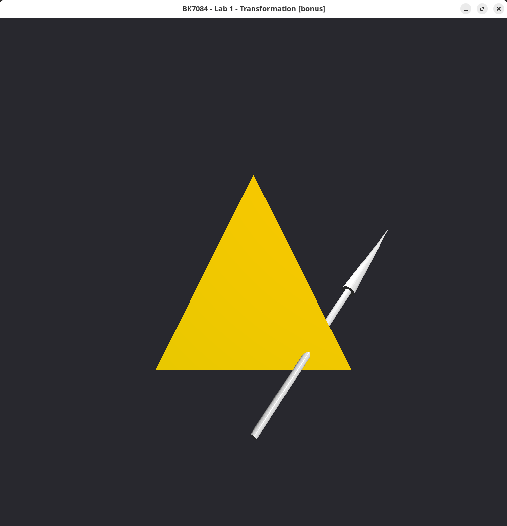
Most of the framework is already implemented for you. When you first run
the exercise you should see a blue triangle with a moving ray (in
green). Your task is to complete the intersection.py file. Once it is
correctly implemented, the triangle will change its color to red when
the ray intersects it.
There are three subtasks, all to be completed in
intersect_ray_triangle:
-
Build matrix A and vector b to create a linear system (see next page).
-
Solve the linear system using NumPy’s solve function:
np.linalg.solve(A, b). -
Implement the intersection conditions based on the solution vecto (see next page).
Ray-Triangle intersection
In lecture 1 we saw the following equation:
\[ \mathbf{r} + t\mathbf{d} = \mathbf{a} + \beta(\mathbf{b} - \mathbf{a}) + \gamma(\mathbf{c}-\mathbf{a}), \label{eq:raytriintersection} \]
where the left side defines a point on a ray and the right side a point on the plane of a triangle. More specifically:
-
The ray is defined by its origin $\mathbf{r}$ and a direction $\mathbf{d}$. The parameter $t$ defines any point along the ray by scaling the direction vector.
-
The triangle is defined by three vertices $\mathbf{a}$, $\mathbf{b}$, and $\mathbf{c}$ and the parameter $\beta$ and $\gamma$ combines the three vertices to define a point on the triangle’s plane.
-
When the following conditions for $\beta$ and $\gamma$ are satisfied, the point is inside the triangle: \[\begin{aligned} \beta \geq 0,
\gamma \geq 0,
\beta + \gamma \leq 1.\end{aligned} \]
We also saw that Equation $\eqref{eq:raytriintersection}$ is actually not one equation, but three: one equation for each axis. We can thus rewrite Equation $\eqref{eq:raytriintersection}$ as:
\[\begin{aligned} r_x + td_x &= a_x + \beta(b_x - a_x) + \gamma(c_x-a_x)\\\\ r_y + td_y &= a_y + \beta(b_y - a_y) + \gamma(c_y-a_y)\\\\ r_z + td_z &= a_z + \beta(b_z - a_z) + \gamma(c_z-a_z) \end{aligned}\]The linear system above contains three unknowns: $\beta$, $\gamma$ and $t$. We have a ray and a triangle, and we want to find a point defined on the plane by the parameters $\beta$, $\gamma$ and the same point defined by the parameter $t$ from the ray. In other words, we want to find $\beta$, $\gamma$ and $t$ that will make the left side of the equations equal the right side. When this happens, we have found a point that is on the ray and at the same time on the plane of the triangle.
Linear systems are commonly expressed in a matrix notation as it makes any computation much simpler. The above equations can then be written as:
\[\begin{bmatrix} a_x-b_x & a_x - c_x & dx \\ a_y-b_y & a_y - c_y & dy \\ a_z-b_z & a_z - c_z & dz \end{bmatrix} \begin{bmatrix} \beta \\ \gamma \\ t \end{bmatrix} = \begin{bmatrix} a_x - r_x \\ a_y - r_y \\ a_z - r_z \end{bmatrix}\]We encourage you to check this. Real understanding comes from working through problems. Try to go from the matrix notation back to the three equations.
We often write the combination of matrices and vectors as
$\mathbf{Ax} = \mathbf{b}$. This is called a linear system. Here, we
know the elements of $\mathbf{A}$ and $\mathbf{b}$, and we want to
find the solution vector $\mathbf{x}$. For our specific ray-triangle
intersection $\mathbf{x} = [\beta, \gamma, t]^\intercal$. One way to
solve this system is by sweeping the matrix (Gaussian elimination). We
will take a shortcut to find a solution by using NumPy’s solver for
linear system. It’s used as follows: x = np.linalg.solve(A, b).